これまでいろいろ遊んできながらもStable Diffusionモデル本体について学んだことがなかったので、ほかに色々遊ぶ前に理解するフェーズを挟もうと思います。
Stable Diffusionは拡散モデルの一種であるLatent Diffusion Model(LDM)をベースとして拡張したモデルです。そのためStable Diffusionモデルの仕組みを知るためにはまず拡散モデルとLDMについて知っておく必要があります。この記事では、拡散モデルとLDMについて簡単に解説した後に、Stable Diffusionそのものの説明に入ろうと思います。
拡散モデルとは何か
まずStable Diffusionにおいて重要な考え方である拡散モデルについて理解します。
We present high quality image synthesis results using diffusion probabilistic models, a class of latent variable models inspired by considerations from nonequilibrium thermodynamics. Our best results are obtained by training on a weighted variational bound designed according to a novel connection between diffusion probabilistic models and denoising score matching with Langevin dynamics, and our models naturally admit a progressive lossy decompression scheme that can be interpreted as a generalization of autoregressive decoding. On the unconditional CIFAR10 dataset, we obtain an Inception score of 9.46 and a state-of-the-art FID score of 3.17. On 256x256 LSUN, we obtain sample quality similar to ProgressiveGAN. Our implementation is available at https://github.com/hojonathanho/diffusion

拡散モデルは元のデータ(例えば、画像や音声)に徐々に「ノイズ」を加え、ほぼ乱数状態になったデータを学習データとし、そこからノイズを取り除いて元のデータを再構成する方法を学習するモデルです。
拡散モデルの基本概念
- 拡散プロセス(Diffusion Process)
- データポイント(画像など)が徐々にランダムなノイズに変換されるプロセスです。
- これは学習過程のみで行われます。
- 逆拡散プロセス(Reverse Diffusion Process):
- ノイズから元のデータを徐々に再構築します。
- 生成モデルはこの逆拡散プロセスを学習し、ランダムなノイズからもそれっぽいデータを生成可能になります。
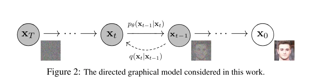
下の画像は拡散モデルの論文から引っ張ってきたものです。この画像が逆拡散プロセスの過程を示しており、これと同じ処理がStable Diffusionでも行われています。
仕組み
- 前向き拡散過程 (Forward Diffusion Process)
- 元のデータ(例: 画像)に徐々にガウスノイズを加えていき、最終的には純粋なノイズにします。
- 元のデータ ( x_0 ) から始まり、各ステップ ( t ) でノイズを追加し、 ( x_t ) を生成します。
- ( x_t = sqrt{1 – beta_t} cdot x_{t-1} + sqrt{beta_t} cdot epsilon_t )
- ( beta_t ) はノイズスケジュール、 ( epsilon_t ) はガウスノイズ
- 逆拡散過程 (Reverse Diffusion Process):
- 前向き拡散過程で生成されたノイズデータから、元のデータを再構築します。
- モデルは、ステップ ( t ) からステップ ( t-1 ) に逆行する条件付き確率分布を学習します。
- ( p_theta(x_{t-1} mid x_t) )
学習方法
- 前向き拡散過程で生成されたノイズデータを使ってモデルを学習します。
- 逆拡散過程の確率分布を正確に近似することを目標として、そのための損失関数が使用されます。
Latent Diffusion Modelとは何か
次にStable DiffusionモデルのベースとなったLatent Diffusion Models(LDM)について説明します。
By decomposing the image formation process into a sequential application of denoising autoencoders, diffusion models (DMs) achieve state-of-the-art synthesis results on image data and beyond. Additionally, their formulation allows for a guiding mechanism to control the image generation process without retraining. However, since these models typically operate directly in pixel space, optimization of powerful DMs often consumes hundreds of GPU days and inference is expensive due to sequential evaluations. To enable DM training on limited computational resources while retaining their quality and flexibility, we apply them in the latent space of powerful pretrained autoencoders. In contrast to previous work, training diffusion models on such a representation allows for the first time to reach a near-optimal point between complexity reduction and detail preservation, greatly boosting visual fidelity. By introducing cross-attention layers into the model architecture, we turn diffusion models into powerful and flexible generators for general conditioning inputs such as text or bounding boxes and high-resolution synthesis becomes possible in a convolutional manner. Our latent diffusion models (LDMs) achieve a new state of the art for image inpainting and highly competitive performance on various tasks, including unconditional image generation, semantic scene synthesis, and super-resolution, while significantly reducing computational requirements compared to pixel-based DMs. Code is available at https://github.com/CompVis/latent-diffusion .
Latent Diffusion Modelは、低次元の潜在空間(Latent Space)で拡散プロセスを行う拡散モデルの一種です。この手法は高次元の画像空間で操作する従来の方法に比べてモデルのパラメーターが少なく済むため、計算コストとメモリ使用量を大幅に削減でき、学習の効率化と画像生成の高速化につながります。
LDMの基本概念
- 潜在空間(Latent Space)
- データの複雑な構造を低次元の潜在空間にマッピングしてから拡散プロセスを行います。
- 画像空間よりもパラメータの少ない潜在空間での拡散プロセスは、計算効率を向上させます。
仕組み
- エンコーダ(Encoder)
- 潜在拡散プロセス(Latent Diffusion Process)
- 潜在変数 ( z ) に対して、通常の拡散プロセスと同様にノイズを加えていきます。
- 前向き拡散過程(拡散モデルと同様)
- (
z_t = sqrt{1 – beta_t} cdot z_{t-1} + sqrt{beta_t} cdot epsilon_t
) - ( beta_t ) はノイズスケジュール、 ( epsilon_t ) はガウスノイズ
- (
- 逆拡散プロセス(Reverse Diffusion Process)
- 潜在空間でのノイズデータから元の潜在変数を再構築します(拡散モデルと同様)。
- モデルは、ステップ ( t ) からステップ ( t-1 ) に逆行する条件付き確率分布を学習します
- (
p_theta(z_{t-1} mid z_t)
) - ここで、 ( theta ) はモデルのパラメータです。
- (
- デコーダ(Decoder)
- 再構築された潜在変数 ( z ) から元の高次元データを生成します。
- – デコーダ ( D ) を使って、潜在変数 ( z ) から再構築されたデータ ( hat{x} ) を得ます
- ( hat{x} = D(z) )
学習方法
- 前向き拡散過程と逆プロセスのトレーニング
- 前向き拡散過程で生成されたノイズデータを使って、逆拡散過程の確率分布を学習します(拡散モデルと同様)。
- 学習の目標は逆拡散過程の確率分布を正確に近似することです。(これも拡散モデルと同様)
Stable Diffusionについて
Stable DiffusionはLDMをベースとした画像生成モデルの実装であり、LDMに学習を効率化、画像生成を高精度化させるためのテクニックを付加したものがStable Diffusionになります。
使用されているテクニックとか
例えば以下のようなテクニックが使われています。
- 変分オートエンコーダ(VAE)
- Stable Diffusionは、変分オートエンコーダ(VAE)を使用して、潜在空間の表現を学習します。VAEはデータの潜在表現を正規分布に近づけるため、安定した潜在空間を提供します。
- クロスアテンション機構
- クロスアテンション機構を導入することで、潜在空間の情報と元の高次元データの情報を効果的に統合します。
- アダプター
- アダプターと呼ばれる小さな学習可能なモジュールをモデルに挿入して微調整を行う方法があり、これはメモリと時間の効率が良く、大規模な計算リソースを必要とせずに効果的なカスタマイズを可能にしています
- LoRAとかがこれです。(言いようによってはAnimateDiffとかも)
- 高速化
- Latent Consistency Models(LCM)などの技術を取り入れることで、Stable Diffusionは最小限の推論ステップで高品質の画像生成を実現できます
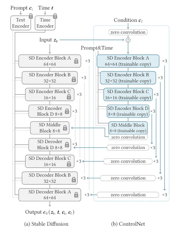
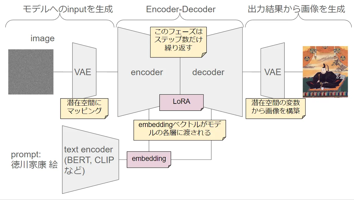
モデルのアーキテクチャ
最後に
触り程度に理解できた気になったのでこれくらいにしておきます。説明がふわっとし過ぎててあまりわからなかった、って方は記事の中に論文へのリンクも貼ってあるので、そこから読んでみてください。
実際に生成を試したい場合はComfyUIをインストールすれば簡単に試せます。以下の記事でインストール手順を紹介しているので読んでみてください。

>-
その他、Stable Diffusion周りで読んだ論文は以下の記事でまとめているので、興味ある方はぜひご活用ください。
Stable Diffusion関連の論文解説記事のリンク集。画像生成・動画生成の基礎モデルから応用技術まで論文ベースで解説。