The Stable Diffusion 3 research paper was published around May, so I decided to take a look.

Following our announcement of the early preview of Stable Diffusion 3, today we are publishing the research paper which outlines the technical details of our upcoming model release, and invite you to sign up for the waitlist to participate in the early preview.

What’s New in the Rectified Flow Model
From what I can tell, the key novelties are roughly the following:
- Improved Text Encoder
- Improved noise scheduler
- Uses techniques like Logit-Normal and Mode sampling instead of the conventional linear schedule
- Introduction of a new Transformer-based architecture (Diffusion Transformer, DiT)
- Demonstrated performance exceeding state-of-the-art models in txt2img
Architecture of the Rectified Flow Model
To summarize briefly: the biggest change is that UNet has been replaced by MM-DiT. Everything else is essentially about increasing model size and parameters to improve performance.
Text Encoder
Previous Stable Diffusion
Used a CLIP text encoder (an encoder pre-trained on large-scale image-text pairs) to encode text prompts and feed them into the image generation model.
Stable Diffusion 3
Uses a combination of CLIP and T5 text encoders: CLIP L/14, OpenCLIP bigG/14, and T5-v1.1-XXL. The outputs from each encoder are concatenated and used together.
UNet
Previous Stable Diffusion
Used the UNet architecture as the core of the generative model — a multi-layer convolutional neural network that performs encoding and decoding of the image.
Stable Diffusion 3
Adopts DiT (Diffusion Transformer) instead of UNet. DiT is a Transformer-based model capable of processing both text and image tokens together. Specifically, it uses MM-DiT (Multimodal-DiT) blocks, which process text and image tokens with separate weights while achieving bidirectional information flow between the two.
VAE
Previous Stable Diffusion
Used a VAE (Variational Autoencoder) to compress images into a low-dimensional latent space, then used those latent representations in the generation process. This enabled efficient image generation and high-resolution output.
Stable Diffusion 3
Similarly uses a pre-trained autoencoder, but the key difference is an increased number of dimensions in the latent space. This improved representational capacity leads to better performance.
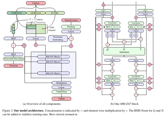
MM-DiT Processing
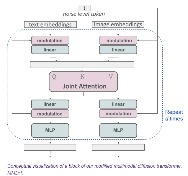
The MM-DiT architecture is designed to handle both text and images. Here is a simplified overview of the processing flow.
Pre-processing
1. Image Encoding (image embedding)
The original RGB image is converted into a low-dimensional latent representation using a pre-trained VAE. The resulting latent representation is split into 2×2 patches along with spatial positional encodings.
2. Text Encoding (text embedding)
Text is converted into embedding vectors using pre-trained models (CLIP and T5). The outputs used are CLIP’s output and T5’s final hidden state.
MM-DiT Block
3. Modulation and Linear Transformation
In multimodal models, it’s important to prevent the model from becoming biased toward any single modality. Adjustments are made through normalization and similar operations to keep values in balance.
- Modulation: Scales embeddings and adjusts bias, using information from a noise level token to adjust processing.
- Note: I couldn’t find an explicit description of the noise level token in the paper, but it likely corresponds to the noise scheduling during training and indicates how much noise is present at the current step.
- Linear: Linearly transforms the embedding vector, compressing its dimensions into a shape suitable for the next input.
4. Concatenation of Latent Representations
The outputs from steps 1 and 2 are concatenated into a single sequence.
5. Joint Attention
The concatenated sequence is fed into QKV Attention, where mutual information is shared between both embeddings to generate an integrated representation.
6. Separation into Text Stream and Image Stream
Since the positions of image and text tokens are clearly defined, the tokens are separated from the attention output back into their original positions.
7. Further Linear Transformation and Modulation
The two streams from step 6 are processed and transformed into a shape suitable for the next MLP. This allows both streams to emphasize their respective features while being adjusted as needed.
Noise Level Token is again used to adjust processing here.
8. MLP
The data after linear transformation and modulation is passed through multiple layers including non-linear transformations for further processing, enabling the learning of more complex features to pass to the next block.
9. Repeat
The entire block process is repeated for as many stacked MM-DiT blocks as there are.
Post-processing
10. Image Generation from Latent Representation
Finally, the latent representation output from the MM-DiT blocks is decoded by the VAE to obtain the image.
Training Method of the Rectified Flow Model (SD3)
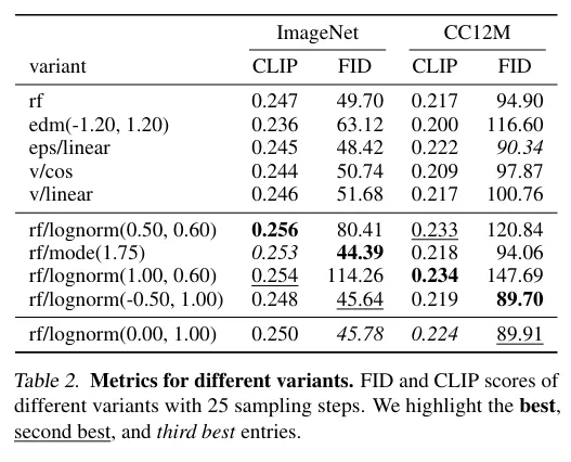
Noise Schedule and Sampling Method
Previous Stable Diffusion
Uses a fixed noise schedule during training (e.g., linear or cosine schedule). Learns to reverse the diffusion process — from noise back to data — through the forward diffusion process from data to noise.
Stable Diffusion 3
The Rectified Flow model introduces a new noise schedule aimed at more efficiently sampling noise at specific timesteps. It uses techniques such as Logit-Normal and Mode sampling to adjust the noise scale, improving training effectiveness at intermediate steps.
Performance Evaluation
The model achieves better scores than existing models on metrics like FID and CLIP. Honestly, just looking at the numbers doesn’t tell me much, so I’ll skip the rest of the evaluation details.
I’ll also quote the generated images from the paper. It appears that prompts written as natural sentences can now be used for generation. Additionally, text is generated without collapse, which is impressive.

Three Model Variants
Stable Diffusion 3 comes in three model variants. The difference between them is likely the number of stacked MM-DiT blocks. The table below shows the parameter counts. The paper mentions 8B parameters for the 38-block case, so Ultra is listed as 38 blocks.
| Model | Block Count | Parameters |
|---|---|---|
| Small | – | 800M |
| Medium | – | 2B |
| Large | – | 4B |
| Ultra | 38 | 8B |
Conclusion
Key points to remember from a user perspective:
- Improved text understanding in the Text Encoder
- Can now interpret sentence-style prompts
- Text generation without collapse looks achievable
- Multimodal (text and image) generation supported by default
- Improved generation accuracy
- Increased parameters and required models
- Likely to be somewhat heavier and slower
There are still parts around the MM-DiT block I haven’t fully grasped, but I feel like I’ve got a solid external view of the model, so I’ll stop reading here for now.
The model was also released recently. Check the article below where I introduce the procedure for using Stable Diffusion 3.

>-
Other papers I’ve read around Stable Diffusion are summarized in the following article — please check it out if you’re interested.
Stable Diffusion関連の論文解説記事のリンク集。画像生成・動画生成の基礎モデルから応用技術まで論文ベースで解説。