Today I explain method to optimize asset allocation of investment portfolio using method called Black-Litterman Model. In this method, combine market data and investor’s view to calculate expected return. In this article, apply Black-Litterman Model actually using Python code, and check the result.
Black-Litterman Model is what
Black-Litterman Model is a model to optimize asset allocation of investment portfolio, developed by Fischer Black and Robert Litterman. This model combines expected return calculated from market data (e.g. stock price or bond return data) and investor’s view (such as analyst’s prediction), to calculate expected return. By performing Mean-Variance Optimization using this expected return, it becomes possible to create portfolio considering both numerically calculated value and investor’s view.
Investor’s view includes investor’s prediction for specific asset or asset group. Prediction of return and uncertainty of that prediction are included. Although saying “Investor’s view”, actually it doesn’t have to be prediction made by human. Therefore, it is also used to blend numerically calculated return with return predicted by machine learning.
Steps to use Black-Litterman Model
- Find Equilibrium Return from Market Portfolio (Reverse Optimization)
- Blend Investor’s View into Equilibrium Return (Bayesian approach)
Step 1: Find Equilibrium Return from Market Portfolio (Reverse Optimization)
Calculate expected return of each asset class calculated from asset ratio and risk of Market Portfolio. State where all investors have same information and evaluation for risk matches is defined as equilibrium, and return obtained in this case is called Equilibrium Return.
Equilibrium Return is found using following formula.
Here risk aversion is indicator of how much investor dislikes taking risk.
Generally, risk aversion is expressed as follows. (Value smaller than 0 is theoretically impossible)
- 0 < delta < 1: Very high risk tolerance (Does not fear risk much)
- 1 < delta < 10: Risk tolerance in normal range
- delta > 10: Very risk aversive (Hates risk very much)
Note: Since it is no problem if expected return can be calculated in this phase, it is also possible to use other models like CAPM.
Step 2: Blend Investor’s View into Equilibrium Return (Bayesian approach)
Calculate expected return combining market information and investor’s view. This equation takes form like below:
Note: is parameter adjusting uncertainty of covariance matrix, seems to be selected by rule of thumb. Generally value of is set small, conversely if investor has own strong view, it tends to be set large.
Formula is complex and makes me want to vomit a bit, but I explain lightly per part.
Left half integrates market equilibrium return and uncertainty of investor’s view, calculating reliability of overall information integrating market information and investor’s view.
- Inverse matrix of sum of reliability of Market Equilibrium Return and reliability of Investor’s View
- Represents reliability of new information integrating prior Market Equilibrium Return and reliability of Investor’s View
Right half calculates new expected return integrating prior market information and investor’s view.
- Integrate Market Equilibrium Return and Investor’s View, calculating new expected return
Finally by calculating , final expected return can be obtained.
Try calculating actually with Python
For simplicity calculate in quite simplified form.
- Assume only Global Stocks and Global Bonds exist in Market Portfolio
Step 1: Find Equilibrium Return from Market Portfolio (Reverse Optimization)
Assume as follows.
Expected return of Global Stock and Global Bond are 5% and 2% Ratio of Global Stock and Global Bond is 60%:40%
Script to calculate Equilibrium Return at this time becomes as follows.
import numpy as np
# Assumption of Market Dataexpected_market_returns = np.array([0.05, 0.02])  # Expected return of Stock and Bondmarket_weights = np.array([0.60, 0.40])  # Ratio of Stock and Bondcov_matrix = np.array([[0.1, 0.02],                       [0.02, 0.08]])  # Covariance Matrix
# Setting Risk Aversion Coefficientrisk_aversion = 2.5  # Assumption of Risk Aversion Coefficient (Actually calculate and find)
# Expected Return of Market Equilibrium Portfolio (\Pi)pi = risk_aversion * np.dot(cov_matrix, market_weights)
print("Expected Return of Market Equilibrium Portfolio (Pi):", pi)
Execution Result
Expected Return of Market Equilibrium Portfolio (Pi): [0.17 0.11]It diverges quite a bit from reality value, but forgive me since it’s hypothetical talk…
Step 2: Blend Investor’s View into Equilibrium Return (Bayesian approach)
First set Investor’s View. Here, predict Stock raises 10% (Uncertainty 4%), Bond raises 3% (Uncertainty 2%) return.
# Investor's Predictioninvestor_views = np.array([0.10, 0.03])
# Uncertainty for View (Covariance Matrix)omega = np.diag([0.04, 0.02])  # Reflect uncertainty of prediction
# Matrix indicating influence of view (Prediction regarding Stock and Bond)P = np.array([[1, 0],              [0, 1]])
Next, calculate expected return of each asset using set Investor’s View
# Setting Scaling Factortau = 0.025
# Calculation of Final Expected Returninv_cov_matrix = np.linalg.inv(tau * cov_matrix)omega_inv = np.linalg.inv(omega)PT_omega_inv_P = np.dot(np.dot(P.T, omega_inv), P)
middle_matrix = np.linalg.inv(inv_cov_matrix + PT_omega_inv_P)part_one = np.dot(inv_cov_matrix, pi)part_two = np.dot(np.dot(P.T, omega_inv), investor_views)final_expected_returns = np.dot(middle_matrix, (part_one + part_two))
print("Final Expected Return:", final_expected_returns)
Execution Result
Final Expected Return: [0.16418829 0.10199786]Compared to result of Step 1, you can see slight correction is entered based on investor’s view.
Final Code
import numpy as np
# Assumption of Market Dataexpected_market_returns = np.array([0.05, 0.02])  # Expected return of Stock and Bondmarket_weights = np.array([0.60, 0.40])  # Ratio of Stock and Bondcov_matrix = np.array([[0.1, 0.02],                       [0.02, 0.08]])  # Covariance Matrix
# Setting Risk Aversion Coefficientrisk_aversion = 2  # Assumption of Risk Aversion Coefficient (Adjustable appropriately)
# Expected Return of Market Equilibrium Portfolio (\Pi)pi = risk_aversion * np.dot(cov_matrix, market_weights)
# Investor's Predictioninvestor_views = np.array([0.10, 0.03])
# Uncertainty for View (Covariance Matrix)omega = np.diag([0.04, 0.02])  # Reflect uncertainty of prediction
# Matrix indicating influence of view (Prediction regarding Stock and Bond)P = np.array([[1, 0],              [0, 1]])
# Setting Scaling Factortau = 0.025
# Calculation of Final Expected Returninv_cov_matrix = np.linalg.inv(tau * cov_matrix)omega_inv = np.linalg.inv(omega)PT_omega_inv_P = np.dot(np.dot(P.T, omega_inv), P)
middle_matrix = np.linalg.inv(inv_cov_matrix + PT_omega_inv_P)part_one = np.dot(inv_cov_matrix, pi)part_two = np.dot(np.dot(P.T, omega_inv), investor_views)final_expected_returns = np.dot(middle_matrix, (part_one + part_two))
print("Expected Return of Market Equilibrium Portfolio (Pi):", pi)print("Final Expected Return:", final_expected_returns)
Conclusion
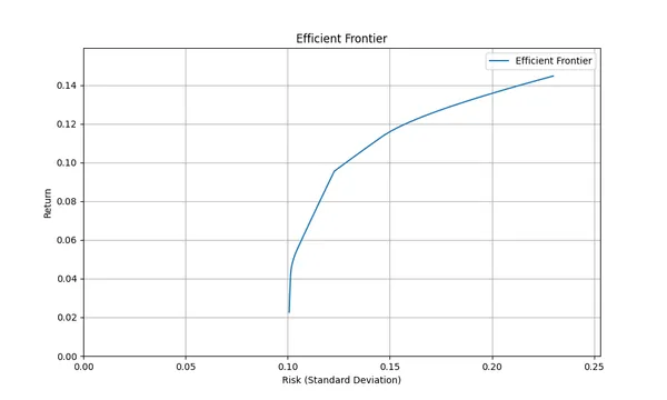
So far we were able to find expected return corrected by Black-Litterman Model. By performing Mean-Variance Optimization using this expected return, optimized efficient portfolio can be created.
Since calculation itself is simple, not much code was needed. Although I skipped this time, I think parts finding Equilibrium Return and bringing Investor’s View become gateway difficulty wise. I think I will check around there and summarize if I feel like it, so I am happy if you come reading again when found.
If you want to know other models related to portfolio construction, please utilize the link collection below.

投資ポートフォリオ構築に関するモデル記事のリンク集。資産配分・期待リターン計算・リスク管理モデルを体系的にまとめています。