Portfolio Diversification: Sector Correlation Analysis in Python

When you want to diversify your stock investments as much as possible, you often wonder which sectors to invest in and how much, right?

Some might say, “Just buy everything in every field,” but that lacks sophistication and can be costly.

This is where correlation analysis comes in handy. Even though sectors are distinct, they often have correlations. By selecting and buying sectors with low correlation, you can obtain the maximum risk diversification effect.

This time, I wrote a Python script to calculate this, so I hope you find it useful. It’s a simple script, so just reading the concept and trying to write it yourself could be a learning experience.

Basic Concept

What is Correlation?

It indicates a statistical relationship showing how much two or more variables are related.

It measures how one variable changes when another variable changes. If one variable tends to increase when the other increases, it’s a positive correlation. If it tends to decrease, it’s a negative correlation.

What is a Correlation Coefficient?

The correlation coefficient takes a value between -1 and 1. Values closer to 1 indicate a strong positive correlation, values closer to -1 indicate a strong negative correlation, and values closer to 0 indicate no correlation.

The calculation method is as follows:

How to Utilize Correlation

If you choose and buy sectors with a positive correlation, it means there is a high probability that when one stock price falls, the other will also fall. This can be said to be a state of high risk against a certain factor.

Conversely, if you choose and buy sectors with a negative correlation, when one stock price rises, the other falls, so returns may be compressed.

Therefore, the idea is to choose sectors that are close to uncorrelated (independent) to gain returns while diversifying risk.

Python Script

Analyzing using all stock prices for each sector is arduous, so we will analyze using ETF data. Returns are calculated over a 30-day period.

Note: To exclude factor returns affecting the entire Japanese stock market, we use a factor model to subtract returns received from TOPIX.

import yfinance as yf
import pandas as pd
import japanize_matplotlib
import seaborn as sns
import matplotlib.pyplot as plt
import numpy as np
from sklearn.linear_model import LinearRegression

# Only one factor for simplicity
def calc_beta(target_return, factor_return):
    # Prepare data
    data = pd.DataFrame({
        'TargetReturn': target_return,
        'FactorReturn': factor_return,
    }).dropna()

    # Prepare for regression analysis
    X = data[['FactorReturn']]  # Explanatory variable
    y = data['TargetReturn'].values  # Objective variable

    # Perform regression analysis
    model = LinearRegression()
    model.fit(X, y)

    beta = model.coef_[0]
    return beta

def calc_unique_return(target_return, factor_return):
    beta = calc_beta(target_return, factor_return)
    unique_return = target_return - beta*factor_return
    return unique_return

# Create a dictionary of ETF ticker symbols
tickers = {
    "TOPIX-17 Foods": "1617.T",
    "TOPIX-17 Energy Resources": "1618.T",
    "TOPIX-17 Construction & Materials": "1619.T",
    "TOPIX-17 Raw Materials & Chemicals": "1620.T",
    "TOPIX-17 Pharmaceutical": "1621.T",
    "TOPIX-17 Automobiles & Transportation Equipment": "1622.T",
    "TOPIX-17 Steel & Nonferrous Metals": "1623.T",
    "TOPIX-17 Machinery": "1624.T",
    "TOPIX-17 Electric Appliances & Precision Instruments": "1625.T",
    "TOPIX-17 IT & Services, Others": "1626.T",
    "TOPIX-17 Electric Power & Gas": "1627.T",
    "TOPIX-17 Transportation & Logistics": "1628.T",
    "TOPIX-17 Commercial & Wholesale Trade": "1629.T",
    "TOPIX-17 Retail Trade": "1630.T",
    "TOPIX-17 Banks": "1631.T",
    "TOPIX-17 Financials (Ex Banks)": "1632.T",
    "TOPIX-17 Real Estate": "1633.T",
    "TOPIX": "^TOPX"
}

# Get stock price data
data = yf.download(list(tickers.values()), start="2009-08-15", end="2024-8-15")['Adj Close']
data.columns = list(tickers.keys())

# Convert to log returns
returns = np.log(data / data.shift(30))

# Extract only TOPIX data
topix_return = returns["TOPIX"]
returns = returns.drop(columns=["TOPIX"])

# Subtract factor returns affecting the entire Japanese stock market using a factor model
unique_returns = returns.apply(calc_unique_return, factor_return = topix_return)

# Calculate correlation coefficient matrix
correlation_matrix = unique_returns.corr()

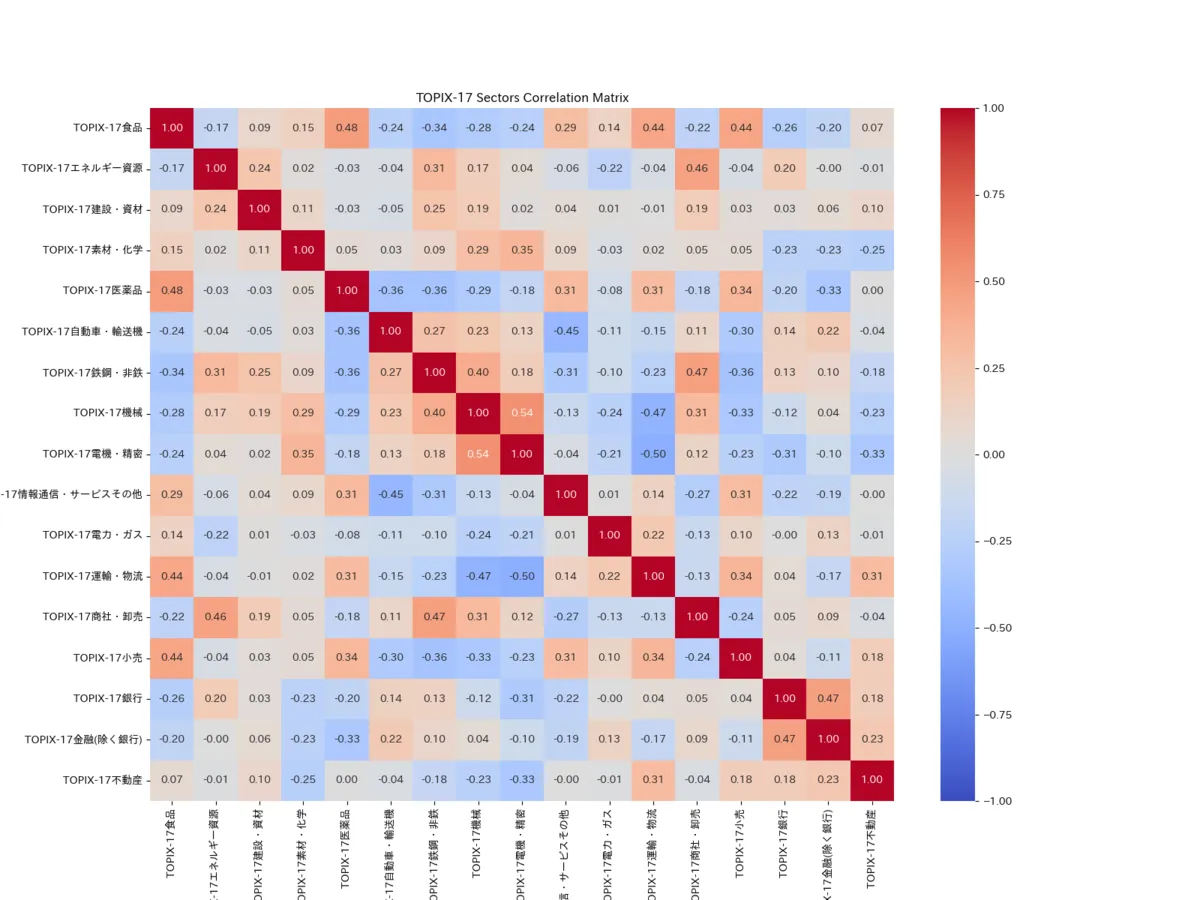
# Visualize with Seaborn heatmap
plt.figure(figsize=(16, 12))
sns.heatmap(correlation_matrix, annot=True, cmap='coolwarm', fmt=".2f", vmin=-1, vmax=1)
plt.title("TOPIX-17 Sectors Correlation Matrix")
plt.savefig("result2.png")
#plt.show()

[Updated 2024/08/31] Fixed because the explanatory variable and objective variable for beta calculation were reversed. The execution result has also been replaced.

Execution Result

The execution result is output as a heatmap. From this, you choose those with correlation coefficients close to 0.

Conclusion

This time, I briefly explained how to perform correlation analysis between sectors using Python. Although I analyzed between sectors this time, this thinking can be utilized in various classification methods such as stocks/bonds, emerging/developed countries, REITs, commodities, exchange rates, etc., so I think it would be good to customize and use it according to your portfolio. Note that dividends and shareholder benefits are not taken into account, so please choose those with good dividends within each sector or consider them separately.

Finally, to add, this itself is just one way of thinking, so rather than operating it alone, it would be better to combine it with other techniques to create a selection method that suits you.

See you in the next article. Bye-bye!