Portfolio Theory with Python: Mean-Variance Optimization Guide

| --- | | Return | Profit obtained by investment. | | Risk | Shows magnitude of return fluctuation, standard deviation of return is used. | | Portfolio | Combination of multiple investments. | | Diversified Investment | Dispersing investment to different assets to reduce risk. This is to suppress influence of failure of specific investment on whole. | | Efficient Frontier | Curve showing optimal combination of risk and return. Portfolios on this curve provide highest return at same risk level. | | Covariance | Indicator showing how much returns of 2 assets link. By combining assets with low covariance, risk of whole portfolio can be reduced. |

Overview of Mean-Variance Optimization

Mean-Variance Optimization is investment theory proposed by Harry Markowitz, calculating risk and return of multiple assets, and deriving how combining them is most efficient.

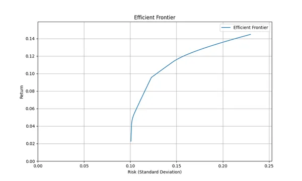
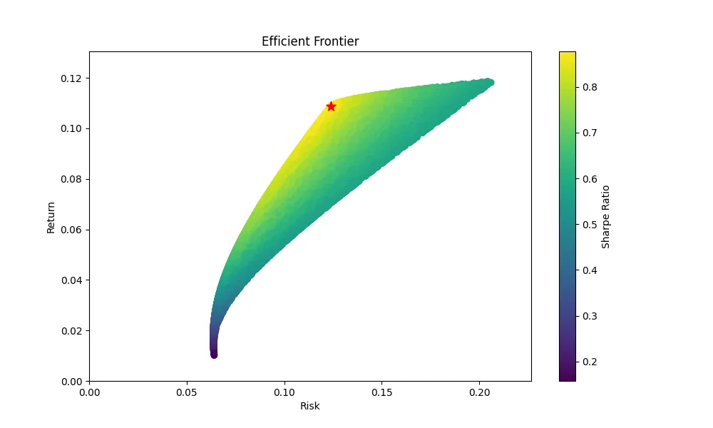
In this theory, curve showing combination of portfolios providing highest return at same risk level is called Efficient Frontier, and it is considered good to buy portfolio on this curve. For example figure below plots risk/return values a certain portfolio can take, curve at upper boundary within this range becomes Efficient Frontier.

And even within Efficient Frontier, point tangent to straight line from origin (star part in figure below) maximizes Sharpe Ratio, so it is said to be most efficient portfolio.

Process of Mean-Variance Optimization

Calculate in flow like below

1. Calculate expected return of each asset
2. Calculate risk (variance) of each asset
3. Calculate covariance between assets.
4. Derive Efficient Frontier based on information calculated in 1~3

Calculation of Expected Return

Various methods like CAPM (other factor models), Machine Learning etc. can be considered for thinking expected return, but since that is not essence this time, I explain with simple method taking average from past returns. Here use log return to consider scale difference by period.

For example, if returns of past 5 years were 5%, 7%, 10%, 3%, 6%, calculate expected return as follows. (Calculate yearly for simplicity)

Calculation of Risk (Variance)

Calculate standard deviation of return. Standard deviation is indicator showing how far return is from average.

Calculation method of standard deviation is as follows:

Calculation of Covariance

General formula to calculate covariance is as follows.

Since I think it’s bit complex, I place example calculating covariance between Asset A and Asset B.

First collect returns of each period. For example assume returns of Asset A and Asset B in past 5 years were as below.

Asset A: 5%, 7%, 10%, 3%, 6%
Asset B: 8%, 5%, 12%, 4%, 7%

Next calculate average return of each asset from return of each period.

Calculate difference between each return and average return, and find their product.

Finally find average of these products (Covariance)

With this, you can know covariance between Asset AB is approx 0.0516%. Since this value is positive, it shows Asset A and Asset B tend to move in same direction.

Construction of Efficient Frontier

This time I show simple method using Monte Carlo method.

To construct Efficient Frontier, use return, risk (variance), covariance matrix of each asset calculated so far. Construct Efficient Frontier in following steps:

First, calculate expected return of portfolio

Next calculate variance of portfolio

Plot standard deviation (x) and return (y) of portfolio on graph.

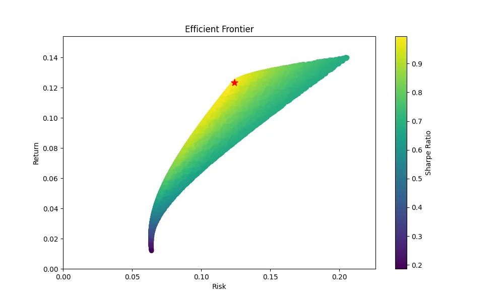
And by repeating work of plotting on graph with various portfolio ratios, range of values (risk, return) portfolio can take emerges on graph (figure below). And upper boundary is portfolio with highest return at each risk level (efficient), that is called Efficient Frontier.

Note: Since Monte Carlo method requires number of trials, but since it can draw Efficient Frontier intuitively, I adopt it here.

Try calculating actually with python

Calculate with simple portfolio composed only of ETFs: VTI, BND, GLDM.

import numpy as np
import pandas as pd
import matplotlib.pyplot as plt
import seaborn as sns
import yfinance as yf

def plot_risk_and_returns(annual_returns, annual_risk):
    # Summarize the results
    summary = pd.DataFrame({
        'Annual Return (%)': annual_returns,
        'Annual Risk (%)': annual_risk
    })
    # Plotting the results
    plt.figure(figsize=(10, 6))
    plt.scatter(summary['Annual Risk (%)'], summary['Annual Return (%)'], color='blue')
    for i, txt in enumerate(summary.index):
        plt.annotate(txt, (summary['Annual Risk (%)'][i], summary['Annual Return (%)'][i]), fontsize=12)
    plt.title('Annual Return vs. Annual Risk')
    plt.xlabel('Annual Risk (%)')
    plt.ylabel('Annual Return (%)')
    plt.grid(True)
    plt.xlim(0, summary['Annual Risk (%)'].max() * 1.1)  # Extend x-axis slightly
    plt.ylim(0, summary['Annual Return (%)'].max() * 1.1)  # Extend y-axis slightly
    plt.savefig("risk_and_returns.png")

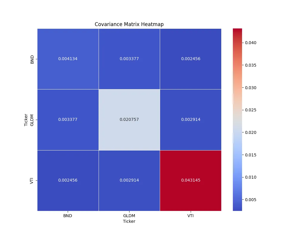
def plot_cov_matrix(cov_matrix):
    # Display the covariance matrix as a heatmap
    plt.figure(figsize=(10, 8))
    sns.heatmap(cov_matrix, annot=True, fmt=".6f", cmap='coolwarm', linewidths=.5)
    plt.title('Covariance Matrix Heatmap')
    plt.savefig("cov_matrix.png")

# Define the tickers
tickers = ['VTI', 'BND','GLDM']

# Fetch historical data for the past 10 years
data = yf.download(tickers, start='2014-05-31', end='2024-05-31')['Adj Close']
log_returns = np.log(data / data.shift(1)).dropna()

# Calculate annual log returns and risk
annual_log_returns = log_returns.mean() * 252
annual_risk = log_returns.std() * np.sqrt(252)
plot_risk_and_returns(annual_log_returns, annual_risk)

# Calculate covariance matrix
cov_matrix = log_returns.cov() * 252
plot_cov_matrix(cov_matrix)

# Monte Carlo simulation
num_portfolios = 100000
results = np.zeros((3 + len(tickers), num_portfolios))
for i in range(num_portfolios):
    weights = np.random.random(len(tickers))
    weights /= np.sum(weights)

    portfolio_return = np.dot(weights, annual_log_returns)
    portfolio_risk = np.sqrt(np.dot(weights.T, np.dot(cov_matrix, weights)))

    results[0, i] = portfolio_return
    results[1, i] = portfolio_risk
    results[2, i] = portfolio_return / portfolio_risk
    for j in range(len(tickers)):
        results[3 + j, i] = weights[j]

# Create DataFrame
columns = ['Return', 'Risk', 'Sharpe Ratio'] + tickers
results_frame = pd.DataFrame(results.T, columns=columns)

# Find the portfolio with the maximum Sharpe Ratio
max_sharpe_idx = results_frame['Sharpe Ratio'].idxmax()
max_sharpe_portfolio = results_frame.loc[max_sharpe_idx]

# Plot efficient frontier
plt.figure(figsize=(10, 6))
plt.scatter(results_frame['Risk'], results_frame['Return'], c=results_frame['Sharpe Ratio'], cmap='viridis')
plt.colorbar(label='Sharpe Ratio')
plt.xlabel('Risk')
plt.ylabel('Return')
plt.title('Efficient Frontier')
plt.scatter(max_sharpe_portfolio['Risk'], max_sharpe_portfolio['Return'], color='red', marker='*', s=100)  # Max Sharpe Ratio point
plt.xlim(0, results_frame['Risk'].max() * 1.1)  # Extend x-axis slightly
plt.ylim(0, results_frame['Return'].max() * 1.1)  # Extend y-axis slightly
plt.savefig("mvo.png")

# Output the portfolio with the maximum Sharpe Ratio
max_sharpe_weights = max_sharpe_portfolio[tickers]
print(f"Max Sharpe Ratio Portfolio Weights:n{max_sharpe_weights}")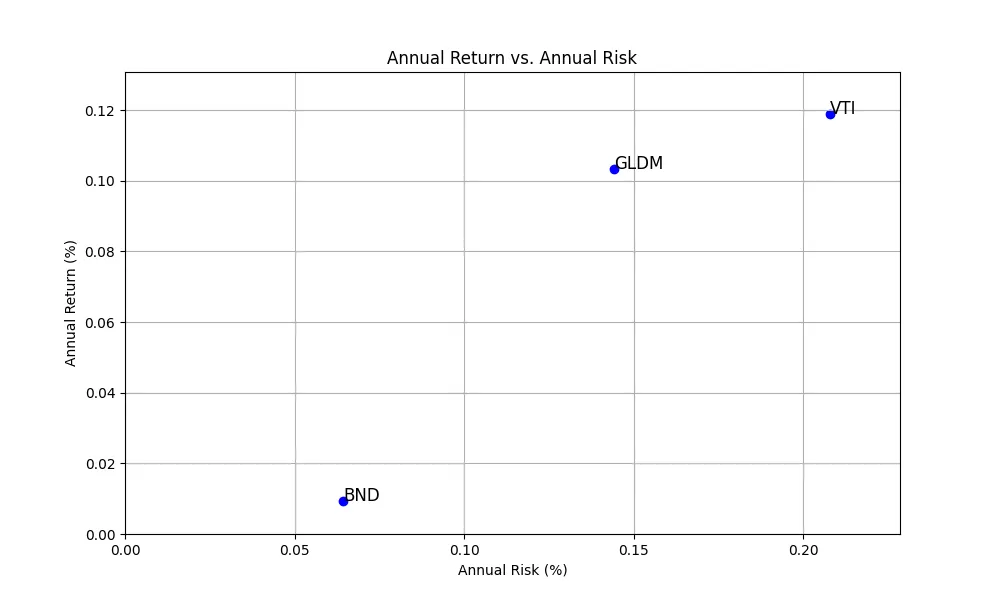

Below is calculated covariance matrix. Diagonal components show variance, others show covariance.

And figure below is Efficient Frontier diagrammed with Monte Carlo method.

Conclusion

I introduced method called Mean-Variance Optimization constructing optimal portfolio combining different assets.

This time for explanation and my understanding, I calculated with simple method, but if solved as optimization problem it can be derived more efficiently, so I will touch that method next.

Note: I touched it

Pythonで解くモダンポートフォリオ理論：平均分散最適化と効率的フロンティアの計算法

>-

blog.otama-playground.com

If you want to know other models related to portfolio construction, please utilize the link collection below.

投資ポートフォリオ構築ガイド: モデル集

投資ポートフォリオ構築に関するモデル記事のリンク集。資産配分・期待リターン計算・リスク管理モデルを体系的にまとめています。

blog.otama-playground.com