In modern investment strategy, many investors focus on risk management of portfolio. Among them, method called “Risk Parity Portfolio” is gathering attention. In this article, I explain basic concept, merit, calculation method of Risk Parity Portfolio, and implementation method in Python.
What is Risk Parity Portfolio
Risk Parity Portfolio is investment strategy aiming to disperse risk of portfolio (i.e. volatility) equally. This strategy is designed so that each asset class has equal risk contribution to entire portfolio. By this, it becomes possible to construct balanced portfolio not depending on specific asset class.
Merit of Risk Parity Portfolio
Main merits of Risk Parity Portfolio are as follows
- Improvement of stability
- Since dispersing risk of different asset classes equally, stable performance not depending on performance of specific asset class can be expected.
- Risk Management
- Risk management of portfolio is easy, and excessive concentration of risk can be avoided. Tolerance to specific market and economic situation improves.
- Reduction of necessity of prediction
- Less need to predict future market trend, and since equalization of risk is basic principle, influence by failure of prediction becomes less.
Demerit of Risk Parity Portfolio
Risk Parity Portfolio also has demerits like below.
- Decrease of Return
- By dispersing risk equally, return of entire portfolio might become low. Compared to strategy investing intensively in specific high risk high return asset, return might become small.
- Especially when incorporating asset with particularly low risk like bonds, there are cases where it becomes almost bonds (depending on situation of correlation).
Calculation Method of Risk Parity Portfolio
In Risk Parity Portfolio, it is set so that risk contribution of each asset becomes equal. And portfolio minimizing sum of squares of difference of risk contribution of each asset is called Risk Parity Portfolio.
Formulate as Optimization Problem
Search weight of asset so that risk contribution of each asset becomes equal.
Objective Function
Constraint
Objective function above is defined to make risk ratio of each asset same following definition of Risk Parity, but can also be expressed using average of risk as below. This objective function aims to bring risk contribution closer to average. (As a result risk ratio of all assets becomes uniform)
Calculation Method of Standard Deviation of Asset
T is number of observation points. Skipping other explanations.
Calculation Method of Covariance Matrix
Skipping explanation here too.
Calculation Method of Risk Contribution
Risk Contribution of Asset i is calculated as follows. Risk contribution indicates ratio occupied by risk of asset in risk of entire portfolio.
Method to calculate Standard Deviation of entire Portfolio
Standard Deviation (Risk) of entire Portfolio is calculated as follows.
Try calculating with Python
Code
import yfinance as yfimport numpy as npimport pandas as pdfrom scipy.optimize import minimizeimport matplotlib.pyplot as plt
# Standard Deviation of entire Portfoliodef sigma_P(w,cov): return np.sqrt((w*cov*w.T)[0,0])
# Risk Contributiondef RC(w,cov): return np.multiply(cov*w.T, w.T)/sigma_P(w,cov)
# Objective Functiondef objective_function(x, params): wt = np.asmatrix(x) cov = params[0] # Standard Deviation of entire Portfolio sig_p = sigma_P(wt, cov) # Risk Contribution per Asset rc = RC(wt, cov) # Target Risk (sigma_P divided by number of assets) target_risk = np.full((1, len(x)), sig_p/len(x)) # Calculation of Objective Function (Multiply 1000 to increase penalty) return sum(np.square(rc - target_risk.T))[0]*1000
def total_weight_constraint(x): return np.sum(x)-1.0
def long_only_constraint(x): return x
# Acquire data and calculate daily returntickers = ['VTI','BND','GLDM']data = yf.download(tickers, start='2021-06-01', end='2024-06-01')['Adj Close']returns = data.pct_change().dropna()
# Calculate Covariance MatrixV = returns.cov().to_numpy()
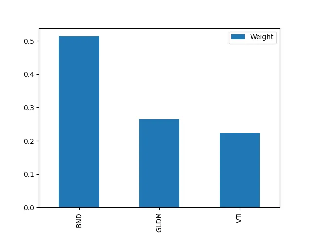
# Optimizenum_assets = len(tickers)w0 = [1 / num_assets for i in range(num_assets)] # Initial value of weightcons = ({'type': 'eq', 'fun': total_weight_constraint},{'type': 'ineq', 'fun': long_only_constraint})res= minimize(objective_function, x0=w0, args=[V], method='SLSQP',constraints=cons, options={'disp': True, 'ftol': 1e-12})w_final = np.asmatrix(res.x)rc_final = RC(np.matrix(w_final), V)w_final = np.array(w_final).flatten()rc_final = np.array(rc_final).flatten()df = pd.DataFrame({'Weight': w_final, 'Risk Contrib': rc_final}, index = data.columns)print(df)plt.figure()df.plot.bar(y = "Weight")plt.savefig('weight.png')plt.figure()df.plot.bar(y = "Risk Contrib")plt.savefig('risk_contrib.png')Execution Result
Weight Risk ContribTickerBND 0.513202 0.001661GLDM 0.263960 0.001661VTI 0.222837 0.001661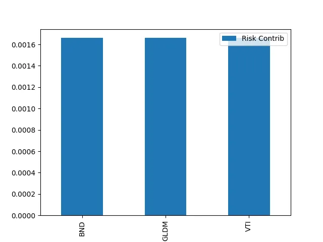
Conclusion
This time I introduced Risk Parity Portfolio. Unlike portfolio emphasizing return introduced before, this portfolio is one conscious of equality of risk. Therefore, return might be less, but since it is equalizing risk per asset, it becomes stable portfolio, so choosing such portfolio according to your life stage is also a choice. Since it is yourself who chooses finally, please consider portfolio suiting you while comparing merit and demerit of each portfolio.
If you want to know other models related to portfolio construction, please utilize the link collection below.

投資ポートフォリオ構築に関するモデル記事のリンク集。資産配分・期待リターン計算・リスク管理モデルを体系的にまとめています。