Modern Portfolio Theory: Mean-Variance Optimization in Python

In a previous article I computed the Efficient Frontier approximately using the Monte Carlo method, but that approach is inefficient — it relies on random sampling and gives different results each run. This time I’ll show how to compute it properly by formulating it as a convex optimization problem using the cvxpy library. The result is exact and reproducible. For a basic explanation of what Mean-Variance Optimization is, see the article below — it’s worth reading first if you’re new to the concept.

Pythonで学ぶモダンポートフォリオ理論：平均分散最適化の考え方

>-

blog.otama-playground.com

Markowitz’s Mean-Variance Optimization Problem

Calculation Method

Among Markowitz’s Mean-Variance models, we solve the optimization problem of minimizing portfolio risk (variance) while ensuring the expected return meets a target value. Specifically, the calculation proceeds as follows.

Objective Function

Constraints

Constraint 1: Expected return equals target value $\mu_p$

Constraint 2: Sum of asset weights equals 1

Constraint 3: Weight is non-negative (no short selling)

Python Implementation

Change the target portfolio return in the code to your own target return before running it.

import yfinance as yf
import pandas as pd
import numpy as np
import cvxpy as cp

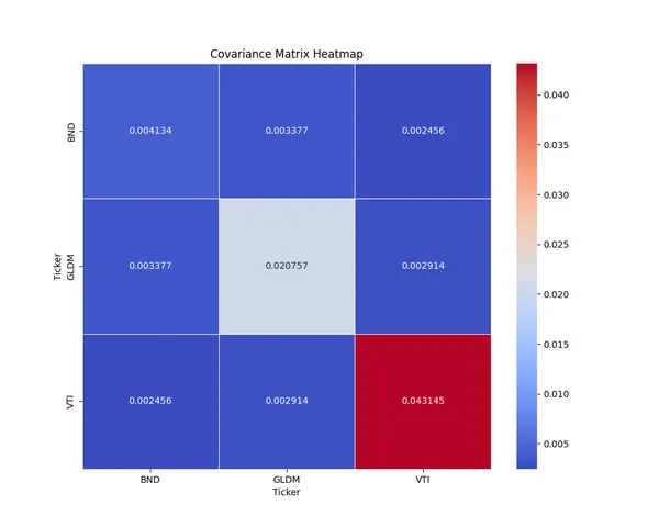
tickers = ['VTI', 'VEA', 'VWO', 'BND', 'HYG', 'EMB', 'IYR', 'GLDM']
data = yf.download(tickers, start="2010-01-01", end="2023-01-01")['Adj Close']
annual_data = data.resample('Y').last()
returns = annual_data.pct_change().dropna()
mu = returns.mean().values
Sigma = returns.cov().values
mu_p = mu.mean()

w = cp.Variable(len(tickers))
objective = cp.Minimize(cp.quad_form(w, Sigma))
constraints = [cp.sum(w) == 1, w @ mu == mu_p, w >= 0]
problem = cp.Problem(objective, constraints)
result = problem.solve()

if w.value is None:
    print("Optimization failed.")
else:
    for ticker, weight in zip(tickers, w.value * 100):
        print(f"{ticker}: {weight:.2f}%")
    print("Expected return:", np.dot(w.value, mu))
    print("Portfolio variance:", np.dot(w.value.T, np.dot(Sigma, w.value)))

Efficient Frontier via Optimization

The Efficient Frontier can also be computed efficiently as an optimization problem — no Monte Carlo needed. The idea is to find the portfolio that maximizes return at each risk level.

Objective Function

Constraints

Python Implementation

To use monthly data instead of annual, change 'Y' to 'M' in the resample call.

import yfinance as yf
import numpy as np
import cvxpy as cp
import matplotlib.pyplot as plt

tickers = ['VTI', 'VEA', 'VWO', 'BND', 'HYG', 'EMB', 'IYR', 'GLDM']
data = yf.download(tickers, start="2010-01-01", end="2023-01-01")['Adj Close']
annual_data = data.resample('Y').last()
returns = annual_data.pct_change().dropna()
mu = returns.mean().values
Sigma = returns.cov().values

target_variances = np.linspace(0, np.max(np.diag(Sigma)), 100)
risks, returns_list = [], []
for tv in target_variances:
    w = cp.Variable(len(tickers))
    problem = cp.Problem(cp.Maximize(w @ mu),
                         [cp.quad_form(w, Sigma) <= tv, cp.sum(w) == 1, w >= 0])
    problem.solve()
    if w.value is not None:
        risks.append(float(np.sqrt(w.value.T @ Sigma @ w.value)))
        returns_list.append(float(w.value @ mu))

plt.plot(risks, returns_list, label='Efficient Frontier')
plt.xlabel('Risk (Standard Deviation)')
plt.ylabel('Return')
plt.title('Efficient Frontier')
plt.legend()
plt.grid(True)
plt.savefig('graph.png')
plt.show()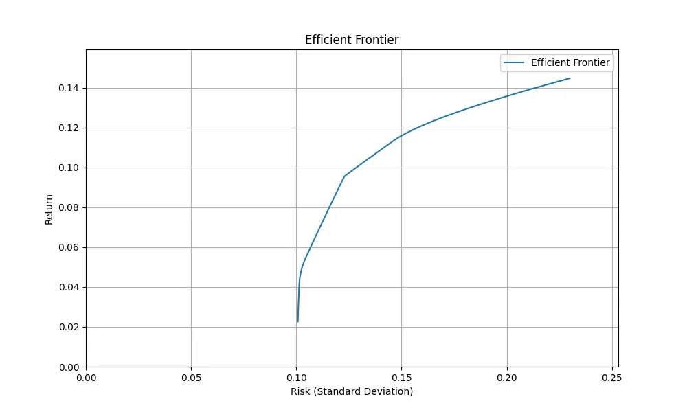

Conclusion

This time I explained how to calculate Mean-Variance Optimization and the Efficient Frontier using Python. These methods form the foundation of Modern Portfolio Theory, and a firm grasp of them should sharpen your investment decision-making. One practical point: the Monte Carlo version is easier to understand intuitively, but the optimization-based version is strictly better for any real use — it’s faster, deterministic, and scales well as you add more assets. I’m still learning myself, so I hope these notes are useful for your own study.

If you want to explore other models related to portfolio construction, please check out the link collection below.

投資ポートフォリオ構築ガイド: モデル集

投資ポートフォリオ構築に関するモデル記事のリンク集。資産配分・期待リターン計算・リスク管理モデルを体系的にまとめています。

blog.otama-playground.com